Training run diagnostic metrics: what I track for when things break down

This post talks a little about the metrics I track to characterize quickly what is going right or wrong with my runs, to save myself precious time and GPU 💸.

To be clear, when I say “break down” I don’t mean the run crashed. That’s a differnt sort of debugging. This is for when the model trains, but it’s not going the way you want it to.

I use Weights & Biases (W&B), but this all applies to similar tools like MLFlow, CometML, and so on.

These metrics are basic, but over the years I’ve picked them up to solve different training run issues. They’re much cheaper to collect and log than doing more runs :)

At the end, I’ll also contextualize how and when I log them in a pseudocode loop. Great for throwing right into a coding LLM as scaffolding for your own projects.

First, let’s talk about the non-negotiables.

📚 The basics, must haves

Obviously you need to set up weights & biases (or whatever you’re using to track with):

1
2
3
4
5
6
7
8
9

if rank == 0:
    wandb.init(
        project=wandb_project_base,
        name=run_name,
        config=checkpoint_config,  # usually a dict with all my keyword args
    )

    # save your config somehow! I like saving the YAML
    wandb.save(config_yaml_path, policy="now")

The simple metrics you MUST track, per step:

1. Learning rate
2. Train loss
   • Per batch
   • Per epoch
3. Test loss
   • Per epoch

These are the foundation of what’s happening to our model over time.

Next, we must agree on our x-axis.

🐾 What is a “step” exactly?

First off, your x-axis for graphs should be the “step” count.

1
2
3
4
5
6
7

# Use our custom "step" as the x-axis for all metrics
# This allows comparing runs at the same training step, even when resuming
wandb.define_metric("step")
wandb.define_metric("*", step_metric="step")

# and then to log each time:
wandb.log({ ... }, step=step)

Each step ends with updating your model’s parameters. So if you are accumulating gradients over multiple forward passes, I would suggest that block being your “step”.

This will smooth out the statistics you report (less noise) and keep all your logic like checkpointing or reporting ticking on the same heartbeat.

An aside: Logging under multiple processes

For a multiple GPU setup, I often will just have a single process reporting back metrics, ie:

1
2

if rank == 0:
    wandb.log({ ... }, step=step)

For training from multiple machines, the advice is similar, you just have to pick a leader somehow.

The only time you need all processes to participate is if you parallelize test set evaluation (which I do).

You’ll need an all-reduce step to “collect” the various losses or metrics from each process, and then combine them to your leader process, which calls wandb.log():

 1
 2
 3
 4
 5
 6
 7
 8
 9
10
11
12
13
14
15
16
17
18
19
20
21
22
23
24
25
26
27
28
29
30

# create our tensor we will all reduce sum over, coming
# from each process in our training process group
# this runs in ALL PROCESSES
loss_t = torch.tensor([
        total_losses['total'],
        total_losses['main_task'],
        total_losses['aux_loss1'], 
        total_losses['aux_loss2'],
        total_losses['aux_loss3'],
        float(num_test_batches_this_process)
    ], device=device
)

# add them all together, elementwise
dist.all_reduce(loss_t, op=dist.ReduceOp.SUM)

# run only on SINGLE process!
if rank == 0:
    # compute averages
    total_test_batches = int(loss_t[5].item())
    avg_losses = {
        'total': loss_t[0].item() / total_test_batches,
        'main_task': loss_t[1].item() / total_test_batches,
        'aux_loss1': loss_t[2].item() / total_test_batches,
        'aux_loss2': loss_t[3].item() / total_test_batches,
        'aux_loss3': loss_t[4].item() / total_test_batches,
    }

    # report back!
    wandb.log(avg_losses, step=step)

To be clear, you can have multiple processes reporting back train metrics. But you’ll end up with multiple data points per step on your graph and this is noisy.

Additionally, with multiple runs it will be harder to compare that metric to a previous run’s if you have multiple lines per run.

With that out of the way, let’s get to the metrics.

🎓 Metric group #1: Grad norm + grad norm per module

You likely already track gradient (grad) norm, what I’ll write as $\left\lVert{G}\right\rVert_2$ since it’s the L2 norm of the gradient before any clipping.

The norm (size) of our gradient basically answers the question: “how large of a change in parameter space is our loss proposing?”

An oversimplification of how the gradient $G$ is applied to your network’s parameters $P$ using learning rate scalar $\alpha$ is:

$$ P_{new} = P_{old} - G_{clipped} * \alpha$$

Note: if your optimizer is something like AdamW, this is directionally but not literally true. Many optimizers try to maintain a “trajectory” of your parameter updates over time (ie: momentum) or other tricks to help you traverse weight-space in a faster manner. But this equation is the underlying dynamic.

where $G$ and $P$ are both vectors of length $N$, the number of parameters in your network.

Grad norm just looks at the sum of all the backwards passes (the gradient) per step (which could be over multiple grad accumulation steps) and concatenates them into one huge, long vector (size $N$) and computes the L2 norm (or length) of it:

 1
 2
 3
 4
 5
 6
 7
 8
 9
10
11
12
13
14
15
16
17

def compute_grad_norm(parameters, norm_type=2):
    """
    Compute the norm of the gradients of the parameters. 

    This implementation computes norms per parameter for memory
    efficiency reasons, rather than concatenating to one giant
    vector and computing the norm on it. The result is mathematically
    equivalent.
    """
    total_norm = 0.0
    for p in parameters:
        if p.grad is not None:
            param_norm = p.grad.data.norm(norm_type)
            total_norm += param_norm.item() ** norm_type
    return total_norm ** (1.0 / norm_type)

grad_norm = compute_grad_norm(model.parameters())

What I propose tracking are additional per-module norms, so for each module of your torch network, you’d compute the subgraph’s grad norm, and also plot that:

 1
 2
 3
 4
 5
 6
 7
 8
 9
10
11
12
13
14
15
16
17
18
19
20
21

def compute_model_grad_norm_per_module(model):
    """
    Compute the norm of the gradients of the parameters 
    for each module in the model

    Returns a wandb-loggable dict with mapping:
        module name: str -> float
    """
    grad_norms = {}
    grad_norms["grad_norm/overall"] = compute_grad_norm(
        model.parameters()
    )
    for name, module in model.named_modules():
        if name and name.strip():
            # Only consider modules with trainable parameters
            if any(p.requires_grad for p in module.parameters()):
                grad_norms[f"grad_norm/{name}"] = \
                    compute_grad_norm(module.parameters())
    return grad_norms

grad_norm_per_module = compute_model_grad_norm_per_module(model)

Why do this?

Well if you track grad norm, it’s because you want to know if network updates are going haywire, either getting too big or too small over time. And if that is the cause, then you’re going to want to know why.

You could easily chalk it up to “oh the learning rate must be too high” or “must be too much regularization” (and it very well might be), but before you go and kick off another expensive run, checking the per-module grad norm can help save you time.

And remember, if you have gradient clipping on, it’s important to track the value pre-clip as that’s the pure signal your learning process is working with before clipping tries to tame it.

Let’s go through a real-world example.

In the below, I was training a small but decently complex transformer network (~11M parameters) for realtime audio. I had just added a number of improvements on the data and architecture side, and kicked off another run.

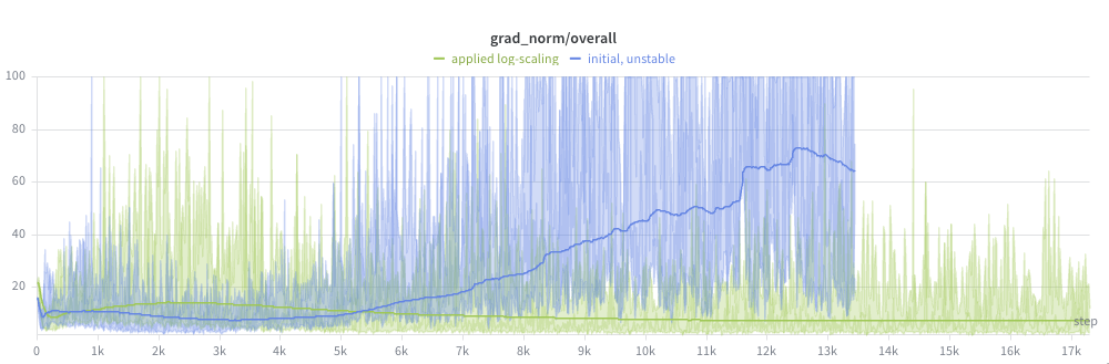
I started to notice the issue with the (pre-clipping) grad norm graph:

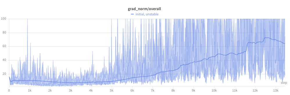
Ouch. This run was not going to converge anytime soon.

And the beginning of the grad norm explosion upwards did coincide with the peak of the learning rate, after the warmup window:

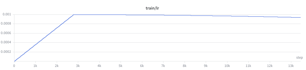
So with the fairly aggressive learning rate of 1e-3, it would be a valid conclusion that the learning rate was too high.

But this didn’t seem right. Even with a bunch of changes, I’d been training this network previously and 1e-3 had proven aggressive, but stable. I hadn’t completely changed the size of the network or regularization in a drastic enough way for this much of a deviation.

Luckily, I had per module grad norm logged!

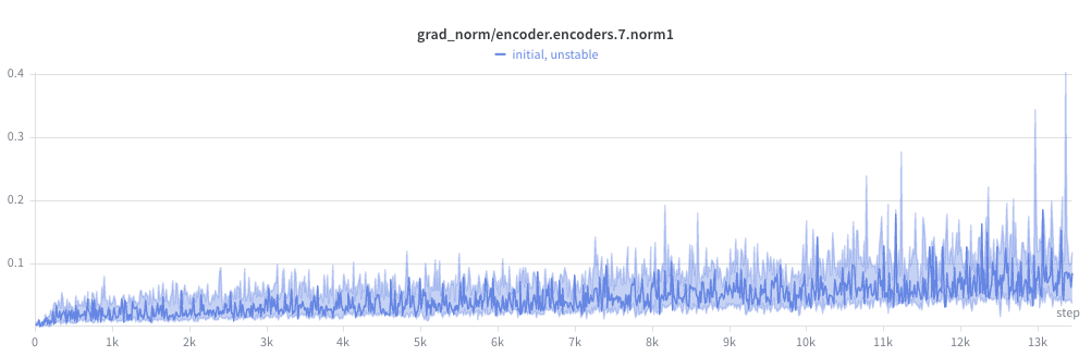
I began to notice a pattern. The gradient norm at later layers seemed high, but not crazy:

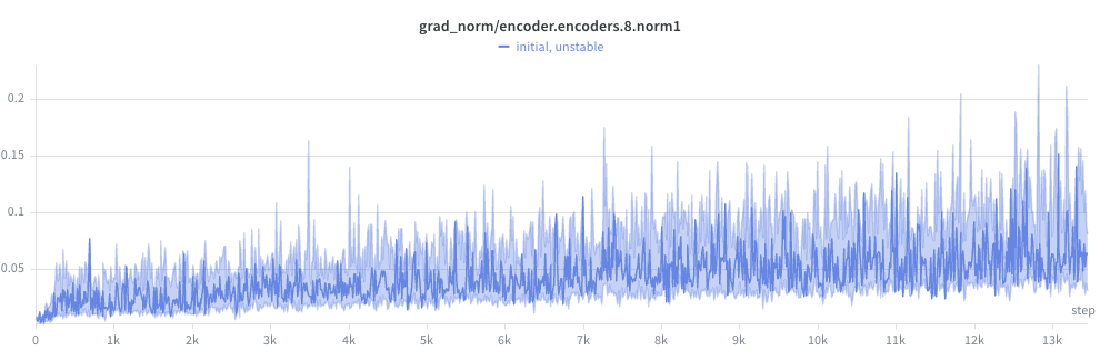
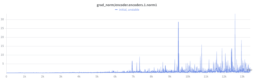
But steadily got worse the closer to the front of the network:

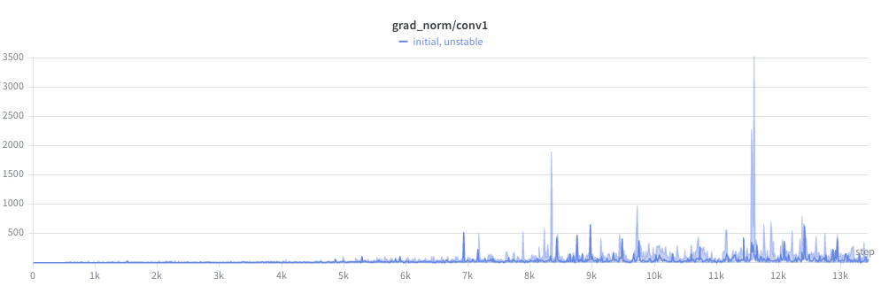
And wild by the first layer (check the y-axis):

But things were totally insane by the frontend conv layers, with peaks in the thousands! For reference, I had gradient clipping on for any gradient norm > 1.0. Clipping prevented the weights from exploding outright, but didn’t fix the underlying problem: the gradient direction was dominated by the unstable parameter, starving the rest of the network of useful gradient signal.

But my conv layers’ random init values seemed completely reasonable. So a dead end there.

But then it hit me.

I had recently hypothesized the model might need to reweight the mel bins based on a loudness curve, sort of like humans have our own auditory perceptual curve (see: Fletcher–Munson equal loudness curve). And in terms of parameters/FLOPs it’s stupidly cheap.

So I added a simple scaling of my mel frames at the start of the forward pass:

 1
 2
 3
 4
 5
 6
 7
 8
 9
10

class Model(nn.Module):
    def __init__(self, ...):
        # ...
        self.mel_scale = nn.Parameter(torch.randn(self.num_mels))
        # ...

    def forward(self, x, ...):
        # x is tensor sized: (batch, time, num_mels)
        x *= self.mel_scale  # hint: don't do this 🤣
        # ...

You might see the train wreck coming.

This had multiple problems:

1. Initialization doesn’t start at identity
   • torch.randn outputs $N(0, 1)$ (gaussian centered at 0)
   • In expectation, now:
     • half our values will be negative (flipping the sign of our features)
     • many are near zero (killing bins entirely)
     • almost none are near 1.0 (identity, passing through original features untouched).
2. Negative values particularly bad for elementwise log-scaling
   • Imagine a mel audio value at a bin of -80 dB. This is virtually silent.
   • Multiplying this by -1 is disastrous. Our quietest bin now is INSANELY loud
   • This is exactly why nn.LayerNorm (and every other normalization layer) initializes its multiplicative weight parameter to ones and its additive bias parameter to zeros. Those are the identity elements for their respective operations.

The fix is very simple.

Multiplying in linear space is addition in log space:

 1
 2
 3
 4
 5
 6
 7
 8
 9
10

class Model(nn.Module):
    def __init__(self, ...):
        # ...
        self.mel_bias = nn.Parameter(torch.zeros(n_mels))
        # ...

    def forward(self, x, ...):
        # x is log-mel, sized: (batch, time, num_mels)
        x += self.mel_bias
        # ...

And we init at 0.0, so this starts as a no-op.

An additional benefit is that because we add self.mel_bias (instead of multiply) our gradient is multiplied by 1.0 instead of the input magnitude, so our gradients (and thus our updates to self.mel_bias) are much more stable.

This completely fixed the issue:

You might also have noticed that because the self.mel_scale scaling tensor was just an nn.Parameter, we wouldn’t get the per-module grad norm computed with the code above. The fix would be to make an nn.Module wrapper for it:

1
2
3
4
5
6
7

class LearnableBias(nn.Module):
    def __init__(self, n_channels: int):
        super().__init__()
        self.bias = nn.Parameter(torch.zeros(n_channels))

    def forward(self, x: torch.Tensor) -> torch.Tensor:
        return x + self.bias

and then compute_model_grad_norm_per_module() would have computed and reported this in the key grad_norm/mel_bias.

Either way, per-module grad norm logging led me to the issue. But without this, I might have wasted another run or two guessing lower learning rates.

And as you know, when you lower the learning rate, it takes you longer to find the issue because the learning process is slowed.

So obviously grad norm per-module is a valuable metric in your toolbox.

Let’s talk about a related measure, the update norm.

📉 Metric group #2: Update norms + effective LR ratio

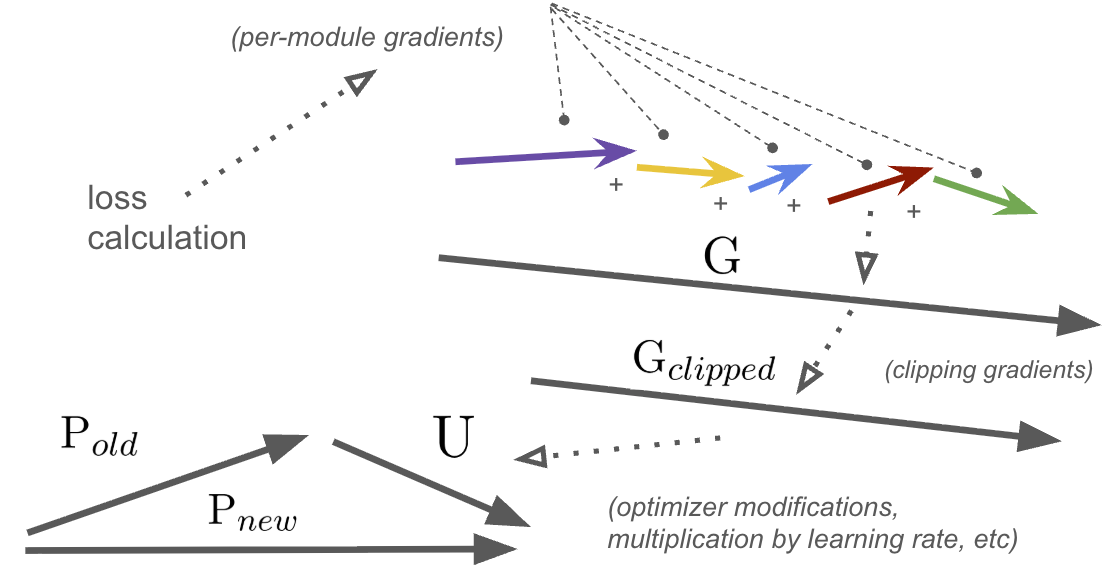
To properly introduce this family of metrics, I drew a diagram:

First, the magic of backprop turns our single scalar loss into a large set of numbers: a gradient associated with each parameter of the network.

We can group the gradient by module into smaller vectors (the colored arrows), which we can characterize for debugging (more on this later).

Finally, we concatenate (not add) them all into a single, much longer vector, $G$ (the gradient vector).

Next, we clip $G$ if necessary, scaling it down to $G_{clipped}$. Note that the direction of $G$ is identical to $G_{clipped}$.

Finally, a bunch of things happen:

• Optimizer modifies $G_{clipped}$ (via momentum, adaptive scaling, etc)
• Learning rate multiplier is applied

These can change both scale and rotation, and gives us the value we actually use to update our parameters. We’ll call it the update, $U$.

And to update the parameters in our network, we apply the standard:

$$ P_{new} = P_{old} - U$$

So from this, we can define a few new metrics:

• Update norm: $\left\lVert{U}\right\rVert_2$
  • “Size” of the actual update in parameter space
• Param norm: $\left\lVert{P_{new}}\right\rVert_2$
  • “Size” of the new model in parameter space
• Relative update norm: ratio of $\left\lVert{U}\right\rVert_2$ / $\left\lVert{P_{new}}\right\rVert_2$
  • How much of the entire network we are changing per-step
• Effective LR ratio: The ratio between the actual step size (update norm) and the gradient norm after clipping: $\left\lVert{U}\right\rVert_2$ / $\left\lVert{G_{clipped}}\right\rVert_2$

Easy, and simple. Here’s how we calculate them:

 1
 2
 3
 4
 5
 6
 7
 8
 9
10
11
12
13
14
15
16
17
18
19
20
21
22
23
24
25
26
27
28
29
30
31
32
33
34
35
36
37
38
39
40
41
42
43
44
45
46
47
48
49
50
51
52
53
54
55
56
57
58
59
60
61
62
63
64
65
66
67
68
69
70
71
72
73
74
75
76
77
78
79
80
81
82
83
84
85
86
87
88
89
90
91
92
93
94
95

def snapshot_params_to_cpu(model):
    """
    Snapshot all trainable parameters to CPU memory.
    
    Use this before optimizer.step() to later compute update norms.
    Copying to CPU avoids GPU VRAM spikes from doubling parameter memory.
    
    Args:
        model: PyTorch model (can be wrapped in DDP)
        
    Returns:
        dict: {param_name: param_tensor_on_cpu} for all requires_grad 
              parameters
    """
    return {
        name: p.detach().clone().cpu()
        for name, p in model.named_parameters() if p.requires_grad
    }

def compute_update_norms(model, old_params_cpu, grad_norm_after_clip=None):
    """
    Compute update norms after an optimizer step.
    
    Measures the actual parameter changes made by the optimizer, which reflects
    the combined effect of gradients, learning rate, momentum, and adaptive
    scaling (e.g., Adam's second moment).
    
    Args:
        model: PyTorch model after optimizer.step()
        old_params_cpu: dict from snapshot_params_to_cpu() taken before step
        grad_norm_after_clip: optional gradient norm after clipping, used to
                              compute effective learning rate ratio
    
    Returns:
        dict with keys:
            - update_norm:
                L2 norm of all parameter changes
            - param_norm:
                L2 norm of all current parameters
            - relative_update_norm:
                update_norm / param_norm (stability metric)
            - effective_lr_ratio:
                update_norm / grad_norm_after_clip (if provided)
    """
    update_deltas = []
    param_flatcats = []
    
    # iterate through new parameters, compare to old
    for name, p in model.named_parameters():
        if p.requires_grad and name in old_params_cpu:
            p_cpu = p.detach().cpu()
            delta = p_cpu - old_params_cpu[name]
            update_deltas.append(delta.flatten())
            param_flatcats.append(p_cpu.flatten())
    
    if not update_deltas:
        return None
    
    update_norm = torch.linalg.vector_norm(torch.cat(update_deltas)).item()
    param_norm = torch.linalg.vector_norm(torch.cat(param_flatcats)).item()
    relative_update_norm = update_norm / (param_norm + 1e-12)
    
    result = {
        "update_norm": update_norm,
        "param_norm": param_norm,
        "relative_update_norm": relative_update_norm,
    }
    
    # Effective LR ratio: shows actual step size relative to gradient
    if grad_norm_after_clip is not None and grad_norm_after_clip > 1e-12:
        result["effective_lr_ratio"] = update_norm / grad_norm_after_clip
    
    return result

old_params_cpu = snapshot_params_to_cpu(model)

grad_clip = 1.5  # just an example
grad_norm_before = torch.nn.utils.clip_grad_norm_(
    model.parameters(), grad_clip
).item()
grad_norm_after = torch.nn.utils.clip_grad_norm_(
    model.parameters(), float('inf')
).item()
grad_clip_ratio = grad_norm_before / grad_clip if grad_clip > 0 else 0.0

# ... etc

optimizer.step()
optimizer.zero_grad()

# .. etc

update_norms_result = compute_update_norms(
    model, old_params_cpu, grad_norm_after_clip=grad_norm_after
)

Interpreting param norm, update norms & effective LR ratio

Reading these metrics together gives a complete picture of training dynamics beyond loss and gradients: where the model is in parameter space, how fast it’s moving, and how much the optimizer is amplifying or dampening the raw gradient signal.

📈 Metric group #3: Non-loss test metrics

This might seem obvious, but I recommend plotting these as well. These might be:

• Accuracy
• Precision / recall / F1 score
• FID score
• … etc

The list goes on.

There are a number of reasons you might want these. After all, the whole point of training this model to you as a human isn’t the loss score, it’s the actual outcomes it allows for!

The other practical reason is that if you change loss formulation midway through training or between runs, you need something objective to judge the performance of the models by in lieu of a loss curve.

Changing your loss formulation can change both the scale and the shape of your loss curve over the course of training.

So yeah, duh. Do it.

🗂️ Metric group #4: Loss by category

Another fairly obvious one, but if you can break out your average loss per batch, per epoch, or per test evaluation by the type of sample, you might be able to find data quality or model parameterization issues.

For example, for a language model you may have different types of queries or chat requests that the model struggles on.

For us, in the music domain, we have found that different genres, stems, or even different bucketed ranges of BPMs gave our models trouble.

So if something is going haywire in a particular category, it can inspire you to do one of the healthiest things you can do in a model training project: actually look at the data!

The solutions for loss discrepancies between categories can range from:

• Correcting data quality issues in those categories
• Adjusting per-sample or per-category weights in some way to bias the model to perform better on those samples (note: do this at the data sampling time, not at loss calculation time if you can)
• Learning that those examples are harder than you thought, and accepting it!

⚠️ Note: if you want to compare loss by category you NEED to make sure you are scaling your loss so that when this measurement is taken, each sample’s loss has the same weight, regardless of length of sample (for sequence models) or quantity of labels.

If you’re just getting less loss because some samples are shorter or have fewer labels, that’s not telling you anything useful about how hard the model is finding that particular category of sample vs another.

One useful pattern for this is using torch’s reduction='none' option when it is available:

 1
 2
 3
 4
 5
 6
 7
 8
 9
10
11
12
13
14

# step 1: calculate per-sample loss for your batch
my_cool_bce_loss = F.binary_cross_entropy_with_logits(
    predictions, targets,
    reduction='none'
)

# step 2: measure raw loss, cut by category, etc
# ...

# step 3: reduction via .mean() to get the actual loss to backprop over 
loss = my_cool_bce_loss.mean()

# step 4: backprop!
loss.backward()

Again, remember to normalize loss for length & label count.

You may also not be able to usefully report per-batch per-category losses if the number of categories is high and you don’t encounter them all every batch. This requires accumulating and reporting these losses every M training steps, every epoch, or every test loop. It’s up to you.

Alright, we’ve covered them all!

Let’s look at a rough sketch of our training loop with respect to all of these metrics.

🔄 Putting it all together: the learning loop sketch

An example of how all this might come together and be structured in a classic train/test loop:

 1
 2
 3
 4
 5
 6
 7
 8
 9
10
11
12
13
14
15
16
17
18
19
20
21
22
23
24
25
26
27
28
29
30
31
32
33
34
35
36
37
38
39
40
41
42
43
44
45
46
47
48
49
50
51
52
53
54
55
56
57
58
59
60
61
62
63
64
65
66
67
68
69
70
71
72
73
74

step = 1
for epoch in range(num_epochs):

    # ── TRAIN ──────────────────────────────────────────────────
    model.train()
    epoch_loss_sum, epoch_steps = 0.0, 0
    accum_loss = 0.0

    for batch_idx, batch in enumerate(train_loader):

        pred = model(batch)
        per_sample_losses = compute_per_sample_losses(pred, batch)
        loss = reduce_losses(per_sample_losses, loss_weights)
        (loss / grad_accum_steps).backward()
        accum_loss += loss.item()

        # ── Optimizer step (every grad_accum_steps batches) ──
        if (batch_idx + 1) % grad_accum_steps == 0:

            # Gradient norms (before clip)
            grad_norms_per_module = compute_grad_norm_per_module(model)

            grad_norm_before = clip_grad_norm_(params, max_norm)
            grad_norm_after  = clip_grad_norm_(params, float('inf'))
            grad_clip_ratio  = grad_norm_before / max_norm

            old_params = snapshot_params_to_cpu(model)

            optimizer.step()
            scheduler.step()
            optimizer.zero_grad()

            # Update norms (after step)
            update_norms = compute_update_norms(
                model, old_params, grad_norm_after_clip=grad_norm_after
            )

            step_loss = accum_loss / grad_accum_steps
            epoch_loss_sum += step_loss
            epoch_steps += 1
            accum_loss = 0.0

            if rank == 0:
                wandb.log({
                    "lr": scheduler.get_last_lr()[0],
                    "train/loss": step_loss,
                    "grad_clip_ratio": grad_clip_ratio,
                    **grad_norms_per_module,
                    **update_norms,
                }, step=step)
            step += 1

    if rank == 0:
        wandb.log({
            "train/loss_epoch": epoch_loss_sum / epoch_steps,
        }, step=step)

    # ── TEST ───────────────────────────────────────────────────
    model.eval()
    with torch.no_grad():
        for batch in test_loader:
            pred = model(batch)
            test_losses = compute_per_sample_losses(pred, batch)
            task_metrics = compute_task_metrics(pred, batch)

    # all_reduce test metrics across processes here (see above)
    if rank == 0:
        wandb.log({
            "test/loss": avg_test_loss,
            **per_category_test_losses,
            **avg_task_metrics,
        }, step=step)

        save_checkpoint(...)

Or something like that. Every train/test loop will be different.

🏁 Summary

Taking the time to instrument metrics for your run takes time, but it will save you much more time when things go wrong!